In this post, I look at a small chart breaking down pay by gender and occupation. Russian wages are particularly flexible, employers have significant freedom in setting the earnings of “inefficient” workers. There’s also a lot of “hidden unemployment”, where workers see their hours deducted at times of low demand (or at the discretion of employers) and where unpaid leave is common. These reasons may contribute to Russia’s gender pay gap.
Gender pay typically varies for several reasons, not all of these are tied to statistical discrimination. Women are more likely to work part-time than men, they also draw to more feminized occupations (like teaching and nursing). Further, women are expected to carry out the bulk of the work tied to parenting, especially in Russia, where traditional gender norms are strongly reinforced. Below, I explore some of these by unpacking pay by gender and occupation. Most noticeably, gender gaps still remain within most occupations, even when limiting the sample to women who work full time (30+ hours per week).
I use the Russian Longitudinal Monitoring Survey for data on participants in 2015. Specifically, I use a measure for gender, occupation, the number of weekly hours worked, and gross wages. I set up the data frame in the following way;
I limit the 4 digit ISCO codes into their most basic categories, for clarity. I also drop those in the armed forces since these are not participating strictly in the labour market. I limit the analysis to women and men who work between thirty and sixty hours per week, although this experience is not representative of all women. The code below outlines the data used. I split earnings by occupation, limit the number of hours worked, drop missing values, calculate mean pay within occupations, and arrange in order of mean pay.
Comparing men and women within occupations reveals significant differences. In almost every occupation, men earn more than women. Surprisingly, the difference is particularly pronounced in Elementary or basic occupations, where pay varies little between workers. Yet in the chart above, men see a roughly 60% advantage over women, almost as high as the men in professional occupations.
For some reason, agricultural workers see almost no difference in pay, possibly because earnings are particularly small in this occupation, where many workers earn the minimum (even lower the women in elementary occupations).
There are other sources of difference worth noting in future posts. Women likely differ by marital status and the number of children in the home, these are the primary sources of gender difference. The tables above only consider all women together. Further, industry differences may play a part in earnings inequality. Women may simply be choosing occupations in less capital intensive industries. These are topics for another post.
This post uses the recent release of the European Social Survey (2016) to revisit public opinion of LGBT relationships. Russia did not participate in the survey since 2012, so this is the first update with wider social data since 2012. This wave also contained some new variables measuring public opinion on Gay and Lesbian relationships, so I decided to revisit the first post.
The previous post had some wider context, so I don’t discuss this here, instead I give some opinions about the data. As before, respondents are given a series of questions about social issues. Their role is to respond in values ranging 1-5; “Strongly Agree” (1) to “Strongly Disagree” (5). These are categorical ordinal variables, so I treat them as categories below. Three question in particular tackle the issue of LGBT rights.
Gay men and lesbians should be free to live their own life as they wish.
If a close family member was a gay man or a lesbian, I would feel ashamed.
Gay male and lesbian couples should have the same rights to adopt children as straight couples.
Taking the first question, I summarise its distribution in Graph 1:
Graph 1: Distribution of LGBT opinion variable by percentage (N = 2200)
.
45% of all respondents strongly disagree with the statement, and the bulk of the data forms either disagreement or strong disagreement with the idea. It seems this variable has changed little since 2012. As noted previously, there may be gender differences in this opinion. It could be that men and women are split on the issue. I tabulate the gender of the respondent against their opinion in the table below.
Table 1: LGBT opinion by Gender
Overall, 47% of men and 43% of women strongly disagree with the statement, and for both genders, disagreement is the most popular option.The results for men and women are almost identical with both genders sharing an equal likelihood of choosing each category. As before, it could be that a spatial element can explain some of the variance. People living in urban settings may be less likely to disagree with the statements than people living in other more conservative parts of the country. At the very least, the Central Area, containing Moscow may be more tolerant of LGBT relationships than other parts of the country. St. Petersburg too, which sits in the North Western Region, may be more tolerant of LGBT relationships.
Percentage of respondents who disagree with the statement by Region
Over 60% of respondents in the central region disagree with the statement. In every region but one, disagreement is the mode. The region least likely to disagree with the statement is the one nearest to Finland, where St.Petersburg is the main city, although here too over 40% of respondents disagree with the claim. Overall, there seems to be little variance in the data, most disagree with the relationship.
Question states: if close family member were gay I would feel ashamed.
The second question too finds strong support for anti-LGBT sentiment, most respondents would feel “ashamed” if a close family member revealed that he or she were gay. The distribution looks similar to the previous variable, and it is unlikely to vary as the previous measure did not.
Lastly, I quickly list the final measure which asks if respondents their opinion on LGBT adoption rights.
Question asks should LGBT couples be allowed to adopt
As with the previous questions, there is a strong anti-LGBT rhetoric in the data. Here disapproval is particularly strong, suggesting respondents with nuanced answers in the previous measures, strongly disagreed with the current measure.
In sum the data has not changed since the previous round of data collection. Because there is so little variance, adding additional variables (like religion) may not be useful. It may be interesting to check who shares egalitarian views, but I will consider this in another post. The results above with have obvious ramifications for Russian citizens, especially LGBT ones, and will likely spill into their working and private lives in other ways.
This post explores the net monthly wages from people’s primary jobs. This data appears in the Russian Longitudinal Monitoring Survey. I sample respondents from 2009 to 2014. For the purpose of the blog post, I just focus on workers who are “currently working”. In the picture below, I summarise net monthly wages in rubles by respondents. The first column “percentiles” lists average monthly wages by percentile. There are 19,000+ observations.
Summary of net monthly wages (in rubles)
The bottom percentile earns just 2000 rubles per month. The smallest value in the percentile is 0. The mean value is 16,500+ rubles, and the median value is 13,000 rubles per month. The upper 1% earns on average 62,000 per month, with the highest monthly wage being 360,000 rubles. The skewness, variance, and kurtosis suggests the data is not normally distributed. This is obvious because wages are never normally distributed. I change wages into a a natural log.
Have wages risen over the last few survey years? I show the distribution of wages in a box and whisker plot by year. Median wages have risen from 2009 to 2014. Variance has fallen slightly since 2012.
Log net monthly wages by survey wave
Have all workers seen a steady rise in pay? I pick 12 random respondents to see how turbulent wages are, I list their wages in natural logs below. Some respondents see no real change in wages like #676 and #28542. Some see sharp declines like #638 and #11995. Lastly, some respondents have seen a year on year rise in pay, like #1156 and #26078.
Log wages of 12 random respondents
As a means of illustrating the values from the random respondents, I illustrate their values over a scatter-plot of all values of log monthly wages divided by the survey year. I also add the average monthly wages by year. The average wages rise very little over the period covered.
Log monthly wages with random individual trajectories and mean trajectory
Lastly, I check who is able to change for “big purchases”. How common do people feel like they’re unable to save for a house, a car, or a larger purchase?
Can you save for a large purchase? 1- yes, 2-no.
77% of observations catch people who don’t not feel like they can save money for a larger purchase. Less than a quarter of all observations capture workers who could save comfortably. I split these observations by income quartiles out of interest. The bottom quartile feels unable to save, 88% of observations feel like they couldn’t put money away for a larger purchase. Interestingly, the top quartile feels only slightly more comfortable with saving, only 38% feel okay with saving.
Quartiles of income by comfort saving for a large purchase.
In this blog post, I wanted to look at trends in vodka consumption. In previous posts, I’ve used the European Social Survey to comment on trends. Recently I’ve been playing around with the RLMS-HSE panel dataset. This is a panel questionnaire that has been running in Russia since 1994. I was trying to use a balanced panel using Stata, and I made some notes on vodka consumption along the way, as an example. I thought I’d summarise some of these here.
Appending the Data
Each “year” (referred to as a “round”) of the RLMS contains a number of variables like gender, income, and other social measures. The data contains a unique ID number (so respondents can be tracked over time) and the year or the round the data was collected. Each variable contains a prefix like “iw”, specific to it’s own round. This prefix just reminds users that the value is specific to a given round. For example the variable “iwdrvodk” asks respondents “Do you drink vodka; yes or no?”. The iw prefix means the variable belongs in the 2014 round of data. I drop this prefix using the code below and save the data to be appended with other years later.
cd "F:\"
global datadir "F:\Russia Panel\study_11735\directory"

use "$datadir/adult2014w",clear


sort idind round
describe idind round iwdrvodk iwgmvodk

rename iw1yago oneyage
renpfix iw

list idind round drvodk gmvodk in 35/50, sepby(idind)
tab round
save "$datadir/trash2014",replace
After getting a number of these individual files ready, I use the Stata command “append” to put a number rounds together. I use the code below to remind Stata that respondents (who are identified using the ID variable “idind”) are followed over time (the years of the survey are identified using the variable “round”), using the command xtset.
append using "$datadir/trash2010"
tab round
append using "$datadir/trash2011"
tab round
append using "$datadir/trash2012"
tab round
append using "$datadir/trash2013"
tab round
append using "$datadir/trash2014"
tab round
xtset idind round
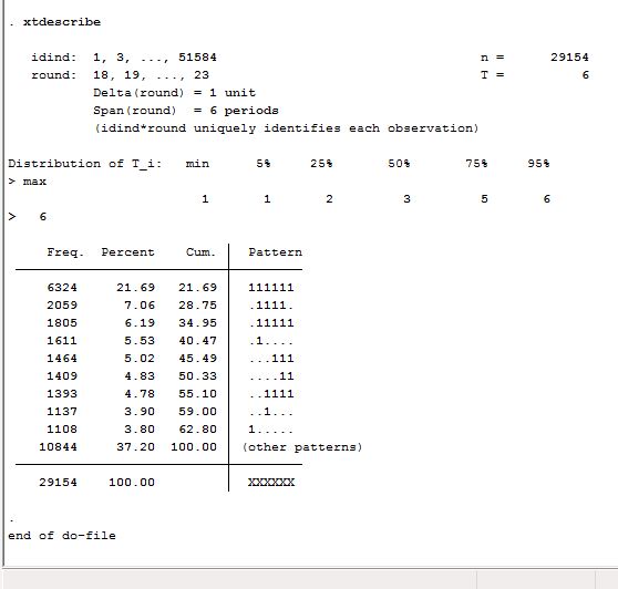
xtdescribe
Once the separate files are merged into one file, I end up with a single person-year file where individuals are followed over time. Not everyone appears in the data set for every round (unbalanced). Some people dip in and out of the survey, but most of the respondents appear six years in a row. I show this in the figure below.
Looking at the figure above, 6,000+ people featured in the panel six years in a row. Several respondents only answered a couple of rounds of data and over 4,000 answered only about one year worth of data. To keep things simple, I focus on respondents who at most, missed only a single round of the survey. I drop the other respondents. In the end, the data looks like this.
In this way, I keep the 6,000+ people who didn’t miss a round, and the 3,000+ people who only missed one round of the survey.
Do you drink vodka?
Right now, the data is structured on two levels. There are observations, or individual answers, and there are people, respondents who are repeatedly measured over time. Questions about vodka vary on both levels, between and within respondents. Ignoring this for the moment, I show the distribution of observations saying yes and no, ignoring the fact that most people answer several times.
The distribution looks about 50/50, but it’s worth asking how it looks “within” people. Below I show how the question “Did you drink vodka in the last thirty days?” varies between and within respondents.
The first column, overall, lists the observations in the data. 12,000+ observations record a “yes”, 13,000+ observations record a “no”. The mode among observations is a “no”. But tells us little about the population, because each person has at least 5 observations, and most respondents have 6. We need a measure that is specific to individuals.
Looking at the “between” column produces a person specific measure. 65% of respondents answered “yes” at least once during the 6 year period. Which is much higher than the observational plot above. 78% of respondents answered “no” at least once during the 6 year period. The total percentage column adds up to over 100% because respondents move between stages of drinking and not drinking. Most respondents claimed not to be drinking vodka at least once during the 6 year period. However, a large portion claimed to be vodka drinkers at least once.
The within column averages the duration of time individuals spent in a given state. Respondents who claimed “yes” roughly spent 66% of their time in the “yes” state. Respondents who claimed “no” roughly spent 71% of their time in the “no” column. The within column just show a measure of “stability” of being in a state. If someone claims they did not drink vodka, they will, on average last longer in the “no” state. However, the respondents who are in the “yes” state still have stability, although respondents tend to leave this category more often than respondents leaving the “no” category.
Basically, there is some movement in and out of being a vodka drinker. I show how this relationship changes over time below using observations which are broken down by time. Since respondents give one observation per year, this should show the trend of vodka consumption over time.
Vodka consumption by year
In 2009, 2010, and 2011 there was roughly a 50/50 split between those who drank vodka and those who didn’t. However the number of drinkers falls by about 5% by 2014 and 2015. The rate of vodka consumption seems to have fallen slightly. However, the tables above break down observations and don’t consider subject specific transitions of being a drinker to not being a drinker (and the other way around). I look at these transitions using the Stata command “xttrans”.
27% of those who said they drank vodka, transitioned into not drinking vodka. However, 27% of those who said they did not drink vodka, transitioned into drinking vodka. The transitions appear roughly even.
How much vodka do you drink?
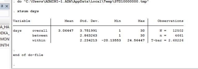
The amount of vodka drunk y respondents also features in the dataset, just like efore this information varies within and between individuals. Obviously, only respondents who drink vodka answer the question about the amount they drink in grams. I summarise this info in the figure below using the command “xtsum”.
The command xtsum, tries to explain the variance within and between respondents. The overall, and within coefficients are counted based on the 12,000+ observations. The coefficient “between” respondents is calculated for the 4,000+ respondents. The average number of rounds (years or points in time) used to calculate these averages is 2.7, which is much lower than the 6 available rounds. Overall the average grams of vodka drunk is 240+. the standard deviation (overall) says that it’s “normal” for an observation to be between roughly 0 and 560 grams of vodka. Basically an observation where someone drinks more than 560 grams is not “normal”. The minimum value says an observation catches someone drinking 3grams of vodka, and somone once drinking 2,000 grams over a thirty day period.
The between column tries to explain that over time, respondents have their own, specific averages. Over the years observed, people’s averages will be located between 3 grams (a ridiculous value) and 1,200 grams (equally crazy) for the entire period. These average deviate by 280 grams of vodka (141*2) and values beyond that are not considered “normal”.
“Grams drunk within respondents” varies between -656g and 1326g. This doesn’t mean that a respondent can drink minus anything, but rather the figure refers to the deviation from a someone’s-specific average. It’s also important to note the overall average is a part of the within cluster minimum and maximum deviations. So the positive deviation of 13oog represents a 1300-243= 1057g maximum deviation that a respondent had from his or her specific average. The maximum deviation that someone had from their overall average is a year where their consumption jumped by 1000g. Luckily this happens rarely between respondents, who overall vary by roughly 280grams. Within respondent habits vary less than difference between respondents in terms of drinking vodka. This just means that a person’s vodka drinking habit varies little over time, but habits between individuals is less predictable.
The average amount of vodka consumed is 200g per month. Between respondents, some drink an average of 3g in 30 days over the period under study, and some drink an average of 1200g over the years over the study. Thinking of the average for each year, I check whether average consumption rises or falls.
In terms of plain observations, the average amount of vodka drunk per year does not vary much. An average person will drink roughly 230-250 grams (if they drink vodka) in 30 days. The chart below shows this using k-distributions.
Vodka consumption by years
On how many days did you drink vodka?
Just like before the number of days respondents spend drinking varies within and between respondents. I summarise this variance below quickly, without getting caught up in the output.
On average, respondents drink vodka for 3 days out of thirty, this probably means respondents just drink over the weekend. This makes sense, since the average amount drank is roughly 200g, typically 4 servings of vodka. This average does not deviate much between respondents the standard deviation is roughly 2 days, which basically means the normal difference between people tends to be about 1 to 7 days, roughly speaking. The average within workers deviates in a similar way, sometimes their average deviated by about two days in a given year, be it plus or minus. In short, this means that following a person over time, sometimes they increase or decrease their days spent drinking by about two days. This is “normal” within respondents. Larger deviations exist in the minimum and maximum deviation but these are several deviations beyond “normal”. I try to show that this rate doesn’t vary much between rounds, although the quality isn’t great. Most respondents spend less than 5 days drinking vodka (if they drink vodka) the majority spend even fewer days doing so.
Number of days drinking vodka
That’s it for now, if someone claims that they drink vodka, their consumption seems to remain steadier within respondents than between respondents. The same can be said for the number of days someone drinks vodka. These figures tend to be more reliable within respondents than between them. If nothing else, hopefully this post has some insight into the Russia Longitudinal Monitoring Survey.
I’m reading “The Economics of Inequality”, and I wanted to check some of the numbers Russia has collected on income share. Once I looked into it I decided to arrange some of the sketches in a small post. Then yesterday, I came across a great article by Ilya Matveev on Russian neoliberalism; discussing how social policy has changed through Kremlin influence and how competition and the market place are affecting not only the welfare state, but education, health and culture. The piece pushed me to put the notes together and post. I really recommend it.
Russia has a flat tax rate, which sets it apart from most European countries. In Piketty’s “Capital” and in “The Economics of Inequality”, he argues that higher rates of taxation on wealth and income are important in the politics of redistribution. Basically if we want to maintain a healthy middle class, we should tax upper rates of wealth and income and redistribute this wealth through public goods like education, health, and welfare policy. Russia does not have a progressive tax on income, and already, as stated in the linked article, things like universal health care for all citizens are in the process of being phased out (or at least these discussions are taking place).
Russia is also a special case as mass market privatization in the early 1990’s made a small group of entrepreneurs extremely rich in a very short amount of time. The state privatised a huge amount of capital to a small group of insiders for heavily discounted prices. Further, Russia has seen a large increase in foreign direct investment, which increased wages for “managers” and those in the finance industry changing the structure of occupations sharply.
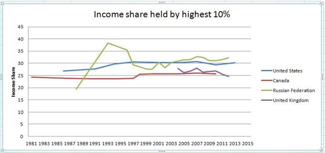
What share of income is held by the top 10%? The World Bank‘s poverty statistics display these stats by country and by year. Russia’s data on the top 10% ranges from 1987, during the time of the Soviet Union to recent years. Some years are missing but generally the series is full. Below, I show the series for Russia’s richest 10% alone. How does their share of income change over time?
The first thing that stands out is the sharp rise in the early 90’s, where a massive deflation of the ruble was followed by a series of privatisation deals as Russia began selling natural resources and other pieces of state capital to private buyers. The decline of income share in the early 90’s could be the result of increased competition as the market adjusted to more “players” (optimistic interpretation) or large amounts of capital flight (pessimistic interpretation). Share of income rises briefly after a large economic crisis in 1998. Most importantly, income share held by the top 10% grows steadily after structural reforms take place, which include a flat tax rate for all citizens (early 2000’s onwards). Only the European recession has affected income share negatively after the reforms, most noticeably the share appears to be growing again. A question worth asking, isn’t this normal? Every society contains inequality, and plenty of other countries have pursued neoliberal policies of growth for far longer than Russia. In the table below, I compare Russia to three other “classically liberal” countries, with limited welfare states and a long history of deregulation of public goods. They are Canada, the US, and the UK.
The first thing to notice is that ultimately, Russia’s richest 10% own a greater share of national income than any other neoliberal example. Despite a gradual rise during the 1980’s the US’ share of national income for the top 10% remains stable, as has Canada’s except for a minor increase in the 1990’s. England’s share, while high, appears to be falling. Adding Denmark to the series (not shows) highlights, that the richest 10% has steadily held on to roughly 20% of national income. In Russia, the richest 10% owns over 30% of all income. How much does the poorest 10% own?
Firstly, Russia’s poorest 10% have one of the lowest shares of national income. The group in Canada and the UK have a greater share of income than the poorest 10% in Russia. The United States is the only country which provides a smaller share. Russia’s series takes a sharp drop during the 1990’s and sees an increase during the late 1990’s. Thinking of the structural reforms, the share in the table above declines quickly shortly after the reforms take place in Russia. The only thing that improves the share of income of the poorest, is the European Recession, after which the share declines again. Ignoring the middle class, how much better are the richest 10% reference to the poorest 10%? I express this difference in a ratio, measuring how many times greater the share of income of the top 10% is reference to those with the bottom 10% of income. The table outlines the trend below.
After the 80’s the richest 10% gain 20 times the income share of the poorest 10%. This gradually declines during the mid 1990’s and increases after structural reforms of the early 2000’s, before stalling and declining during the recession.
Ultimately, Russia’s income inequality is on par with liberal nations like the US and the UK. Structural reforms which were meant to improve life for the middle class, have affected the income of the poorest 10% negatively and improved the income share of the top 10%. Flat taxes are also likely contributing to this trend.
The state of Russia’s economy has been a strong talking point in the media recently, especially with the announcement that GDP will stall this year, along with the prediction that 2017 will be a particularly hard one for Russia if crude oil prices remain low, and sanctions remain in place.
UPDATE; I’ve been playing with this data for a couple of days, writing and taking things out of the post. In that time the ruble has suffered quite a bit, I’m aware of this.
On the upside, Russia is responding to pressure by continuing its investment in technology, and some of the numbers looking at software exports seem positive. That being said, I’m not an economist. I’m more interested in how these “predictions of hardship” are divided up among Russia’s citizens. Since the poverty rate has been rising steadily since sanctions were put in place, it’s safe to say that not everyone feels the pinch equally.
In this blog post I’ll explore “satisfaction with the economy”, looking at how opinion is divided by education, political ideology, and some other variables. In the previous post, I just listed some tables, but here I’ll finish with a small regression table to highlight what are some important variables for citizens who think about the economy. A small disclaimer; the results are meant to be descriptive and aren’t really generalizable. I’m just splitting up the relationships found in the data. I use the weights provided to try to give an accurate representation of Russia, but I don’t have time to make some of the bigger decisions like transforming the dependent variable and checking residuals, so it’s safer to just think about the regression output as a thought experiment, which I may expand on another time.
As in the previous post, I use the 2012 round of the European Social Survey, I haven’t had time to download other waves and this is the most recent one available on Russia. Obviously the data is cross sectional since I’m looking at one year. In the future I want to combine some of the waves and check whether working classes change their opinion of the economy when it shows signs of growth.
What was 2012 like for Russia? The economy was growing, some argued it was the fastest growing economy in Europe, but crude oil prices were high, a graph of the index is shown below;
2012 Figures for crude oil
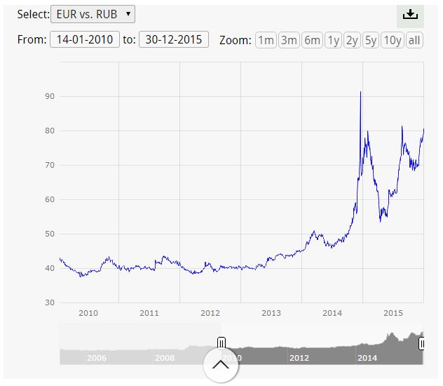
In 2012 crude oil prices stayed at roughly $95 per barrel with some variance, there was a minor fall in oil prices in 2011, but mostly price remained over $80 per barrel, a sign of stability. Another important indicator is the price of the ruble, which at the time hovered about 40 rubles to a Euro, give or take. There were no major changes that year either, and very little variance in ruble price, at least that’s my opinion anyway. An index of the ruble-euro price is shown below.
Ruble- Euro exchange
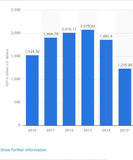
Lastly, I should outline Russian GDP, which saw some increases in early 2010 before seeing declines in 2013. A histogram of GDP in billions can be found below, all I’m trying to use it for is to outline that Russia was experiencing a perfectly normal economic year in 2012. Here’s the graph.
Okay, again I’m not an economist and I’m much more concerned with Russians’ lived experiences and their ability to plan for the future. Overall 2012 was a steady year in Russia’s development. My question now is were people satisfied with the economy and how was that satisfaction divided?
I imagine those who watched a lot of news were probably happy with the economy, and individuals who had good jobs were also satisfied with how things were being run. Although times of economic prosperity should show less variance in satisfaction with the economy, (since everyone is doing well they tend to group together on a high mark) my guess is that Russia’s inequality tends to divide the “spoils” of economic stability. This can be said for most unequal societies. In 2012 Russia had the same Gini coefficient as the United States for inequality, so wealth was distributed roughly evenly in both countries. Basically, I would think that the less “well off” Russians are more likely to be unsatisfied with the economy, while better off citizens would be happier with the several years of stability.
The variable for “satisfaction with the economy” is outlined below;
Histogram of variable “Satisfaction with the Economy”
Surprisingly, the respondents lean towards disapproval of how the economy is managed. Only a very minor group of respondents are “extremely satisfied”. There some to be three major distributions here, a group that are extremely dissatisfied, dissatisfied, and those with minor satisfaction, or maybe indifference. I also split the distribution into a table;
Roughly 78% of respondents are either unsatisfied or indifferent with the economy, this is surprising because Russia had a particularly stable years in 2010, 2011, and 2012. How is this opinion divided by political party?
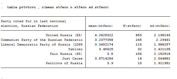
Mean satisfaction divided by party last voted for
Looking at the table above the average score of each political choice was disapproval with the economy. The bulk of votes at “0” is likely skewing the results somewhat, but even United Russia, the party in power, voters collectively averaged at disapproval of the way the economy is run. LDPR and the Communist group had the lowest scores, which may be down to ideological differences. The fringe groups have values closer to United Russia, and are unlikely to be statistically different from those voters.
Thinking of respondent education, I outline their approval of the economy by higghest qualification;
Satisfaction by education
Regarding education, a number of things emerge. Firstly, there is also a dominant lean towards disapproval, no collective group is on average satisfied with the way the economy is run. Secondly the more education acquired, the less satisfied respondents were with the economy. A notable exception here is the group with only a vocational degree, that have particularly low satisfaction levels and low training. The lowest level of economic satisfaction was among those with doctoral degrees, although the group is notably small and can be influenced by extreme values.
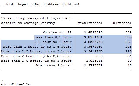
Satisfaction divided by time spent watching the news
A common criticisms of Russia states that people are indifferent to the country’s woes because they watch a lot of uncritical TV. Pundits argue that Russians often see one sided news and politics; therefore, they tend to ignore the obvious bad signs around them in favour of the government’s line. Actually, if we break down opinion by the amount of news people consume, we see people who watch more news are less satisfied with the state of the economy, compared to those who watch less news. It’s important to keep in mind that people who watch a lot of news are often people who have little else to do, and may be vulnerable in terms of being unemployed etcetera. Basically, if someone’s watching a lot of TV, the reason why they’re worried about the economy is because they have a lot of free time on their hands.
Satisfaction with economy broken down by political interest
Another proxy for “attentiveness” might be political interest, a table averaging out “satisfaction with the economy” can be found above. There’s a slight correlation here, highlighting that those who are interested in politics are less satisfied with the economy. Yet again, approval of the way the economy is being run cannot be isolated using this variable. In fact this can be said for all of the variables used. SO far, no group has been isolated as one that approves of the economy.
Thinking of “trust in politicians”, we see a pretty strong statistically significant correlation between those who trust politicians and those who approve of the economy. It may be worth looking at “political trust” to see how common trust in politicians is.
Trust in politicians
In 2012, trust in politicians was extremely low, I don’t want to dwell on this for now, because it’s likely a discussion for another blog post; but basically, satisfaction with the economy is roughly as rare as trust in politicians. This might mean that Russians lack trust in public institutions, again, more on this later. It might be worth breaking down the averages of “satisfaction in the economy” by trust in politicians.
Here, I show a slightly clearer version of the correlation above (with out the significance test). The greater the trust, the greater the satisfaction. However, again an important thing to keep in mind, is that some of the highest values in political trust only average at the most basic values for economy satisfaction; the large cluster of values at “0” for satisfaction with the economy is probably affecting this.
Model for satisfaction with the economy
The visibility isn’t great here, I’m still trying to figure out how to work WordPress, but this small model tries to predict a person’s satisfaction with the economy; looking at the constant (_cons) the value for the model when all the other variables are at zero, is 2.5, so very low satisfaction with the economy. Going through the list, it seems that certain variables “trump” others in terms of predicting a person’s satisfaction with the Russian economy. Here, I’m looking at P-values (P>|t|). P values are described by Charles Wheelan as the probability of gaining a value as high as the one you’ve received, in a scenario where no relationship exists between the variable and the dependent variable. Anyway, more on P-values here. In the model I proposed above, the most important values are “left/right scale”, a square of “left/right scale”, some categories of “TV viewing” in reference to no TV viewing, some political parties voted for relative to United Russia, and “trust in politicians”. The variables that are insignificant in the model are education, and feelings about household income. This is a bit disappointing as I thought that those struggling would report dissatisfaction, and those that are more educated would report dissatisfaction, but anyway.
People who are more right wing are more likely to be satisfied with the way the economy is being run, or at least they were in 2012. There’s also a squared effect, this means that people at the extreme ends of the scale are less likely to be satisfied with the economy. After a certain point, those moving towards the right begin to disapprove of the way the economy is being run.
In terms of TV viewing, those who watch a lot of TV are likely to be dissatisfied with the economy; however this is likely to be the result of those who have no employment, or who part time.
Communist party, and Zhirinovsky’s LDPR voters were significantly more likely to disapprove of how the economy was being run. However, it’s important to note that the other parties had very small bundles of voters, there were very few people in those categories, even before they were fit into the model.
Trust in politicians increased their likelihood of approval for the economy.
In summary, the people who approved of the economy were few and far between, they were mostly United Russia voters, or a voter for a party other than the communist party or LDPR. With a greater sample size, it’s likely these differences would fade. Education doesn’t play an impact when considering the other variables, but in the cross tabs above, there’s a slight suggestion that more educated voters are unhappy with economic management. Right wing ideologies approve of the economy more than left wing respondents, although an effect at the tail ends of both ideologies exists.
Surprisingly, the education variable revealed no result, neither did “feelings about household income”. In fact, the strongest variable predicting a respondent’s “feelings about the economy was trust in politicians”.
Overall in the 2012 sample, there was disapproval of economic management, despite a relatively positive year for the country.
In my first post, I’d like to outline some of the ways LGBT opinion differs in Russian society, using some simple tables and crosstabs. Russia is often described as a country unaccommodating of LGBT relationships. In June 2013, the country’s child protection laws were changed to punish the promotion of “non-traditional sexual relationships”. Although same sex relationship were decriminalised in 1993, Russia is often described as a conservative country with little empathy for LGBT lifestyles. I try to explore public opinion of LGBT rights below and find some nuance.
The European Social Survey collects social statistics, creating generalisable samples of several countries every 2 years or so. Russia took part in the process in 2006, 2008, 2010, and 2012. I’m using the 2012 sample to talk about the country. Regarding LGBT rights, respondents were asked whether they agreed with the statement “Gays and lesbians should be free to live as they wish”. I outline the variable below;
LGBT rights; frequency and percent
I’m not considering missing values in the table above. Some people didn’t know how they felt about the issue, some people left the question blank. I don’t discuss these answers, because I’m more concerned with formed opinions. Thinking of the chart above, there was strong disapproval of gay and lesbian freedoms in 2012. Only 23% of respondents agreed or strongly agreed that they should be left to live “as they wish”. Further to this, the most popular opinion was strong disagreement with LGBT freedom.
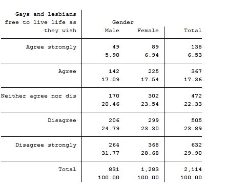
LGBT opinion divided by gender
Dividing the pattern by gender, I outline more of the same. Approval is unpopular with men and women displaying equal favour of “strongly disagreeing” with the statement.
LGBT issues are often portrayed as a political topic, with pundits loyal to one side dividing their opinion based on the party line. I outline this argument here, it’s possible that people in Russia identify more often as right wing, or conservative. A greater number of conservative groups, means fewer people to empathise with LGBT rights. Here, I use placement on the political Left to Right scale, an 11 point scale which asks people whether they are conservative or liberal. I break down the average political score per answer to the LGBT question.
Average placement on the Left-Right scale by LGBT opinion
Looking at the chart above, there’s little indication to suggest that disagreement with the statement is the result of political ideology. There’s no difference in strong agreement or strong disagreement in terms of political ideology.
Another idea worth considering is the divide between urban and rural areas. Urban cities like Moscow and St. Petersburg may be more accommodating of LGBT relationships, and therefore people in these places might be more accepting of LGBT lives. The “Region” variable maps out the locations where individuals were interviewed, the codes are outlined below;
St. Petersburg and it’s surrounding areas are located in RU12, with Moscow and it’s surrounding areas located in RU11. From there the codes move eastward towards Khabarovsk and Kamchatka (RU 18). A crosstab listing the distribution of LGBT opinion by region is outlined below;
LGBT opinion by Region
In every region the “mode” in opinion appears to be “disapproval/strong disapproval”. Moscow appears to be the only region where “Neither approval nor disapproval” is listed as the mode. It also seems like the further east the survey moves, the more conservative the answers become, with the Caucus region being an area of considerable interests. Strong disagreement can be found there, with no respondents “strongly agreeing” with LGBT freedoms.
Lastly, I quickly check the average age of each opinion. Are younger people more likely to agree with the idea that LGBT individuals should live “as they wish”?
There’s a minor age effect present in the variable, the older individuals get, the more likely they are to disagree with the statement. However, those who are agreeing with LGBT rights are not exclusively young, the average age is 40 for both categories. Strong disagreement is strongly dominated by older respondents.
Overall the picture emerging here, is of strong disapproval of LGBT lifestyles. This disapproval seems to have some regional effects, but it is very minor. No region believed that LGBT rights should be standard or at least, no region thought mostly favourably of LGB rights. This issue doesn’t look like a political one either, as respondents with strong beliefs about LGBT freedoms didn’t place differently on the left-right scale compared to respondents who disapproved by LGBT freedoms. Men and women also felt similarly in the propensity to dismiss LGBT issues.
Thinking of the context is important here, especially because the data is only collected in 2012. I’m not looking at shifts and falls in approval over time, only at the data present in one time. In 2012 Russia was just “debating” the gay-propaganda fines and how they would take effect, it’s possible that discussions and debates on the issue were watched on TV and listened to on the radio. These may have shaped opinion towards disapproval.
There are further steps I’d like to take here, I’d like to look at educational differences and check their effects. I also think that religiosity may be having an impact here. Overall there was strong disapproval for LGBT relationships, and isolating the group that approves of the lifestyle wasn’t possible in the charts above.